Page 166 - 应用声学2019年第4期

626 2019 年 7 月

0 0
1540
10 10
20 20
1535
30
30 40
๒ງ/m 40 1530 ๒ງ/m 50
50
60 1525 60
70
70 80
80 1520 90
90 100
1515 1520 1525 1530 1535 1540 1545
200 400 600 800 1000 1200
ܦᤴ/(mSs -1 )
௑ᫎ/min
图 4 背景声速剖面集
图 3 连续检测到的声速剖面伪彩图
Fig. 3 Pseudo-color map of continuous monitor- Fig. 4 Sound speed profile
ing of the sound speed profile

0
60
50 20

40 40
ࣨए 30 ๒ງ/m 60

20
80 EOF1
EOF2
10
EOF3
100
0 -0.2 -0.1 0 0.1
0 5 10 15 20 25
ܦᤴ੸ү/(mSs -1 )
ྲढ़ϙ᫽஝
图 6 前三阶经验正交函数
图 5 声速起伏矩阵协方差矩阵的特征值分布
Fig. 6 Empirical orthogonal function of first three
Fig. 5 Eigenvalue distribution of covariance ma-
order
trix of sound velocity volatility matrix
0 1540
2 声速剖面水平变化对声场的影响
1538
10
2.1 海深不变模型
声速剖面是声场构建的重要参数之一，对于声 ๒ງ/m 20 1536
速剖面水平变化对声场影响的研究有助于地声参 1534
数反演、声场重构等。设仿真海深为 40 m，最大传 30
1532
播距离为 80 km，在0 m ∼ 80 km内，声速剖面跃层
深度变化规律为 40 1530
10 20 30 40 50 60 70
r
( ) ᡰሏ/km
z(r, t) = z(r 0 ) + 1.5 cos 2π − ωt , (10)
13
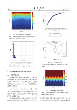
图 7 声速剖面随距离变化伪彩图
其中，z(r 0 )是参考距离上起始时刻的跃层深度，r 为
Fig. 7 Pseudo-color map of sound speed profile
距离，单位为 km。根据以上规律，得到声速剖面随 with distance variation
距离变化如图7所示。
运用RAM模型对声场进行仿真，对于水平均匀 两种模型的海洋参数等除声速剖面外保持一致。其
声场，采用接收位置处的声速剖面进行仿真，其中， 中，声源深度为 20 m；接收深度为 15 m；接收距离